The Name Similarity Vortex

Wait for it…

Is that even possible? How many combinations are we talking about?

library(babynames)
library(dplyr)
all_names <- babynames %>% 
  select(name) %>%
  distinct()
num_names <- as.numeric(nrow(all_names))
# We want to combine every name with every other name
# but we're not interested in every name with itself (- num_names)
# and we can assume the similarity between A and B is the same
# as the similarity between B and A (divide by 2)
((num_names * num_names) - num_names) / 2.0

## [1] 4734569395

That is a lot of combinations! How would we even generate all of them? Luckily Colin Fay created tidystringdist to do just that.

library(tidystringdist)
lots_of_names <- tidy_comb_all(all_names, name)

## Error in matrix(r, nrow = len.r, ncol = count): invalid 'ncol' value (too large or NA)

Oh no! what happened there!? Well, the thing is 4 billion combinations is really a lot (like really a lot!). The maximum amount R can handle is 2147483647 (.Machine$integer.max). But maybe we don’t want all combinations. It is likely that most combinations won’t meet our similarity threshold so we could filter these out. That means we can use furrr!

library(furrr)
library(stringdist)

calculate_similarity <- function(the_name, lots_of_names){
  lots_of_names %>% 
    mutate(weight=stringsim(the_name, name, method='lv'), 
           from=the_name, to=name) %>%
    filter(weight>0.8, weight != 1.0) %>%
    select(from, to, weight) -> result
  return(result)
}

plan(multiprocess)
result <- future_map_dfr(all_names$name, ~calculate_similarity(.x, all_names))

The furrr package allows you to parallelize a lot of the purrr-functions. And it only takes one extra line of code! However, we’re not finished just yet. The result has duplicates:

result %>% 
  filter(from %in% c("Elizabeth", "Elizabith") 
         & to %in% c("Elizabeth", "Elizabith"))

## # A tibble: 2 x 3
##   from      to        weight
##   <chr>     <chr>      <dbl>
## 1 Elizabeth Elizabith  0.889
## 2 Elizabith Elizabeth  0.889

As I said in one of the above code chunks we can assume that the similarity between A and B will be the same as B and A so we only need one of the two. However removing these duplicates is not easy but that’s why we have StackOverflow. The solution by Thomas Leeper uses some good ol’ R code which I found hard to decipher so I broke it up in some dplyr and furrr statements.

# original solution: 
# result[!duplicated(apply(result,1,function(x) paste(sort(x),collapse=''))),]

# first combine the two names into a character vector
result %>% mutate(id = future_map2(from, to, ~c(.x, .y)),
                  # then sort the names
                  id = future_map(id, sort),
                  # then paste the names together 
                  id = future_map_chr(id, paste0, collapse="")) %>% 
  # then remove duplicates
  distinct(id, .keep_all = TRUE) %>%
  select(-id) -> result_unique

Oof! A lot of work but I managed to reduce the number of records from 4734569395 to 591108 (in result) to 295554 (in result_unique).

The knee bone connected to thigh bone

Now that I have my desired output I can finally create my humungous graph (80787 nodes and 295554 edges, no problem right?).

library(tidygraph)
library(ggraph)

result_graph <- as_tbl_graph(result_unique)

result_graph %>%
  ggraph(layout='kk') +
  geom_edge_link() + 
  geom_node_point() +
  theme_void()

Turns out creating a very large graph is not something R is suitable for. Firstly, calculating the layout is computationally hard with this many nodes and edges. Secondly, plotting it in such a way that it doesn’t look like a hairball or spaghetti is near impossible.

One way to overcome this problem is to reduce the size of the data. For graphs this means creating clusters of nodes or communities and igraph includes a number of clustering algorithms. Since I don’t know what I’m doing here I’ll just copy/paste code I found at this StackOverflow question. After playing around with some of the algorithms, I settled for cluster_walktrap.

library(igraph)
communities <- cluster_walktrap(result_graph, 
                                weights = E(result_graph)$weight)

The clustering has resulted in 5538 communities with a skewed size distribution. The largest community has 11904 members and there are 4717 communities with less than 10 members. Let’s explore some of the communities.

Using the igraph functions membership and induced.subgraph we can select specific communities and plot them. I’ll show the code for one plot and forego it for the others.

create_sub_graph <- function(group){
  subg <- induced.subgraph(result_graph, which(membership(communities) == group))

  subg %>%
    as_tbl_graph() %>% 
    ggraph(layout='kk', weight=1/E(.)$weight) + 
    geom_edge_link(aes(start_cap = label_rect(node1.name), 
                       end_cap = label_rect(node2.name))) + 
    geom_node_label(aes(label=name)) +
    theme_void()
}

create_sub_graph(1)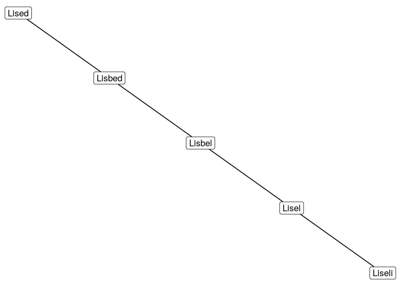

That looks quite boring, I think we can do better.

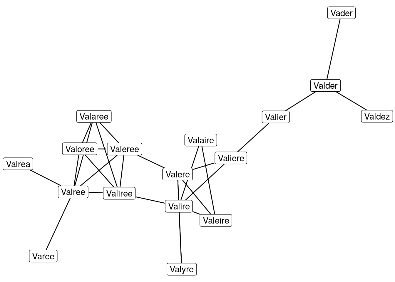
That’s a bit better, with more members the graph starts to look interesting. Let’s ramp it up.

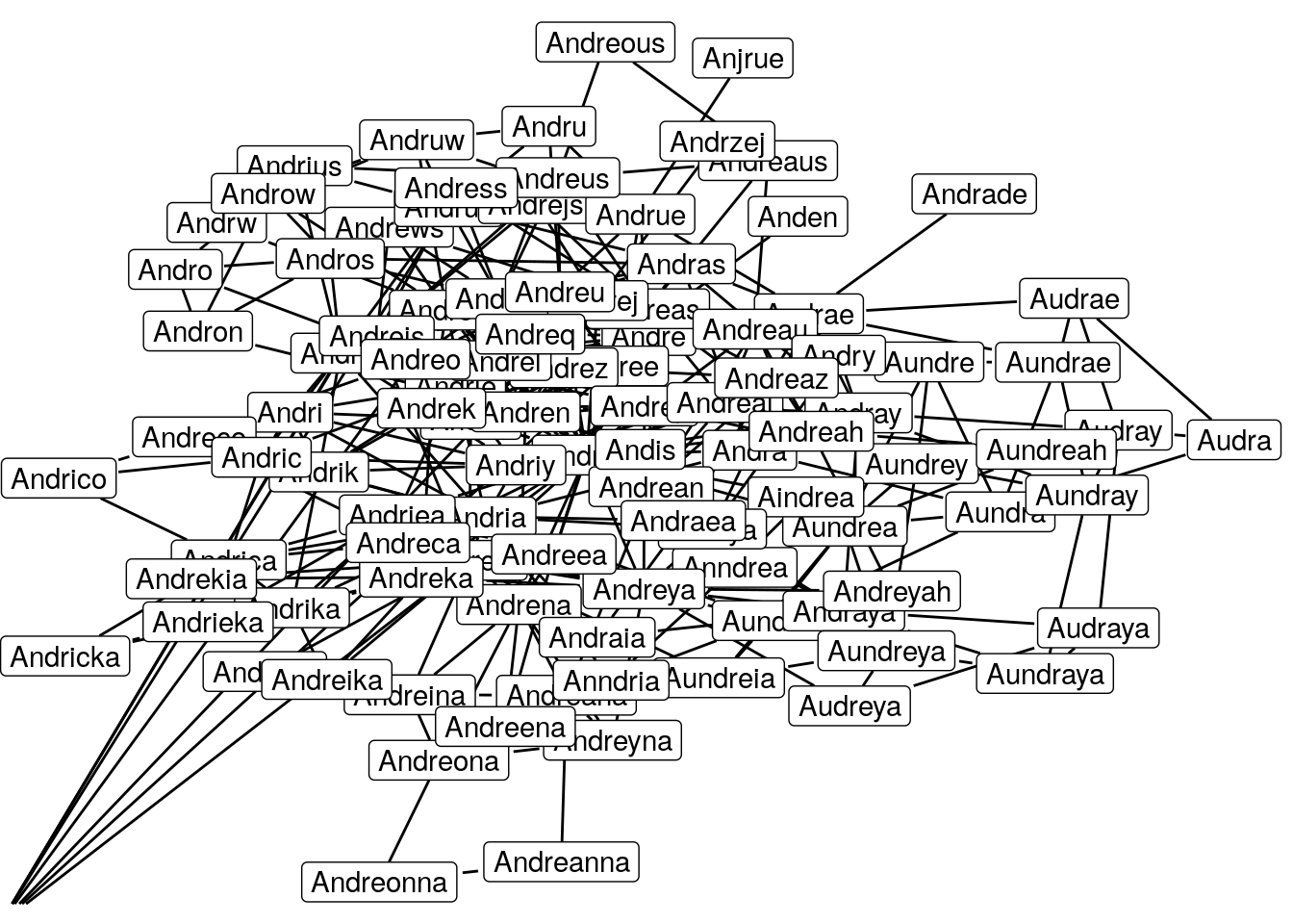
Woooow that kind of hurts the eyes doesn’t it. I think I reached the limit of what is still readable but perhaps I have crossed the limit of what is still understandable.

Enter the vortex

At this point I would still like to know what a plot of all the communities would look like. So using the communities object I can now reduce the size of the original graph, which is what the next code block is for.

# We use the communities object to combine nodes from the same community
# and make sure only one edge exists between two communities
result_graph %>%
  contract(membership(communities)) %>%
  simplify() %>%
  as_tbl_graph() -> comm_graph

The graph is much smaller now, with only 5538 nodes and 1.083910^{4} edges. I’ll use the same code for creating graphs so far except now I’ll just use points rather than labels and I’ll use the size of the communities for the colour and size of the points.

comm_graph %>%
  activate(nodes) %>% 
  mutate(num_names = purrr::map_int(name, length)) -> comm_graph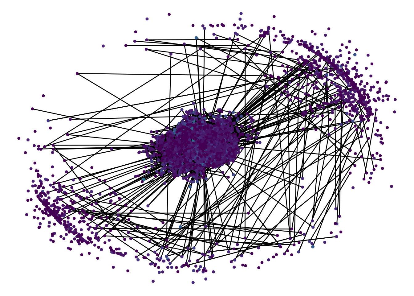

There it is! The Name Similarity Vortex. Isn’t it a beauty? Sit back for a bit and admire it’s hypnotising attraction.

I was hoping for a more meaningful graph but the size distribution of the communities is so skewed that the large number of small communities sort of get in the way. It is interesting to see that the outer ring on the graph is formed by small communities that are not strongly related to any other community.

I played around with other approaches to handle large graphs such as multidimensional scaling (as per David Selby’s instructions) but I just ended up with more nodes and edges. I guess the names are just too intertwined to visualize neatly.

Vortices are the new wormholes

After having discovered The Name Similarity Vortex I can now safely retire babynames. I still have a few ideas but that will have to wait for future blogposts.

Now if you don’t mind I have to go and do some genetic mutation with a snake. Tune in for the next blogpost to find out about the result.